Spectroscopic Applications in Astronomy

 Astronomy and Archaeology are very similar professions in a way that the subject of study in both cases are neither in the vicinity of the researcher in space nor happening in the present time. The only way that people in these professions can work is by making a story out of the little bits of information that reaches them and then verify those stories on the basis of scientific and logical correctness. Life is easy as a chemist when you can mix two chemicals in your lab and watch the reaction unfold or as a biologist when you can dissect an insect to study its anatomy. Nonetheless, this very art of storytelling is what makes Astronomy so fruitful and satisfying. When you are able to determine the chemical composition of a star thousands of light years away or calculate the velocity of a galaxy. Except in the study of nearby planets and meteorites, it is not feasible to receive material information from astronomical sources. We have sent human missions to the Moon to take soil samples. Sometimes we receive a meteor from the outer worlds that carry valuable elemental and physical information. We have sent probes further to transmit information back and some to return with samples from celestial bodies. Perhaps, in the next few decades we will send a probe to the nearest star. What about the countably infinite stars and galaxies that stretches across the night sky? Presently, the most common way by which information reaches us from distant astronomical sources is in the form of Light or Electromagnetic Radiation.

We are constantly showered with electromagnetic waves and cosmic rays from the sky. They are the most fundamental way by which we perceive information from the Universe; constituting of periodic disturbances in the electric and magnetic field, the existence of these waves was first properly suggested by James K. Maxwell through his famous Maxwell’s Equations. Today, we know a lot about the nature of light. From the classical wave nature to the quantum particle nature, light comes in all sorts of colors and energies. The 19^th and 20^th century was a wonderful time for Astronomy and Physics as parallel breakthroughs in these fields were taking place almost simultaneously. These groundbreaking discoveries were facilitated by each other and contributed to a lot of the Modern Physics we know today.

The most important moment in Astronomy was when physicists decided to take a prism and point it at the light coming from the Sun. A prism is a special optical device made of glass, which splits white light into its constituent colors – Violet, Indigo, Blue, Green, Yellow, Orange, and Red. Each of these colors of light differ in terms of their wavelengths and frequencies which is the distance between two consecutive peaks or troughs of the waves and the number of oscillations in one second respectively. The light of red color has the greatest wavelength and least frequency while violet color has the least wavelength and highest frequency. Although their frequencies and wavelength differ, all of the colors travel at the same speed of 3 lakh kilometers per second. In 20^th century, an important discovery in Quantum Physics proved that the energy of a photon is directly proportional to its wavelength and further that light isn’t emitted or absorbed continuously but in discrete chunks of energy. This meant that blue light has more energy as compared to say red light. However, the spectrum of electromagnetic radiations is not just limited between Violet and Red. It extends further on either ends into the more energetic Ultraviolet, X-Rays and Gamma Rays and the less energetic Infrared, Microwaves and Radio waves. 

Fig 1 : Dispersion of White Light by a Prism

The study of hot gases was pivotal in the development of early Astronomy. In the simplest language possible, if one takes any element in a gaseous state(hydrogen for e.g.) at low energies and subjects it to a polychromatic (multiple wavelengths) light source. The spectrum of such light source obtained after passing it through a prism has a characteristic property. This spectrum when viewed on a screen can be observed to have vertical dark lines at specific positions(Fig 2). The normal spectrum of white light indicates lights of different frequencies (color) from left to right. Each position on that spectrum corresponds to a light of a specific frequency. Although the spectrum is made of continuous bands, we can slice its portion into vertical lines, with each line representing a fixed frequency. Therefore, in the second spectrum obtained after passing the light through hydrogen gas and then the prism, the observed dark lines indicate absence of light of that frequency. Since, those dark lines are observed only when hydrogen gas is present in the path of light, it can easily be concluded that gaseous hydrogen is absorbing some of the light of specific frequencies only. The quantum explanation for this is that each atom of hydrogen in that gas is composed of two parts – the central, positively charged nucleus and the negatively charged electrons orbiting it. These electrons orbit the nucleus at fixed energy levels at a certain distance from the nucleus. Most of the times, an electron can absorb energy either in the form of light or heat and jump up to the higher energy level. However, the electron has to absorb that energy which is perfectly equal to the energy difference between the two levels. In case of light, this would mean it can absorb only those photons whose frequency corresponds to that energy difference.

It is as if, there are molds of specific shapes which take in a continuous fluid to form shapes like triangle, circle, etc. whilst leaving the same shaped gaps in the fluid. This spectrum of light after passing it through a cold fluid of specific elements is known as the – “Absorption spectrum” of that element. The absorption spectrum of each element is unique and is characterized by the position of dark lines in that spectrum. Thus, by observing the signature absorption spectra of elements one could determine the name of that element. What if we repeat the same experiment but this time, instead of a light source we heat up the hydrogen gas and energize it. As you might have guessed, this will have the opposite effect as compared to the absorption spectra. When the gas is energized, electrons in the atoms of that gas jump down from higher energy levels to lower energy levels. In order to conserve the energy, the atom emits a photon (light particle) having the same energy as the energy difference between the two levels. If you now observe the spectrum of light coming from such an energized gas, you would observe vertical lines of fixed frequencies against a completely black background. The lines are of a single color (monochromatic), indicating that the hydrogen gas only emitted light of specific frequencies. Furthermore, as one might expect, these color lines are exactly at the same position in the spectrum where the dark lines are observed in the absorption spectrum. This spectrum obtained from the light emitted by a hot or energized element is known as the “Emission Spectrum” of that element. If you overlap the emission spectrum of an element over its absorption spectrum, then the position of dark and colored lines would perfectly coincide and you would retrieve the ordinary spectrum of white light. The final take away from this is that every element can absorb or emit light at specific frequencies, this result in absorption or emission spectra of different elements which is unique for every element.

Fig 2 : Ordinary spectrum of white light vs Emission and Absorption Spectrum of an element.

Returning to the story of stars: In the 19^th century, Joseph Fraunhofer who was a German physicist and an optician analyzed the spectrum of light coming from our Sun and many other stars. He mounted a prism to the eyepiece of his telescope and pointed the telescope at those stars. To his surprise, Fraunhofer noticed vertical, dark lines in those spectra at specific positions. He precisely labeled the set of these dark lines according to their positions, which became known as “Fraunhofer lines”. Many years later, the similarity of Fraunhofer lines to the absorption spectra of certain gaseous elements was discovered. The implication was clear, there was a presence of these gaseous elements in those stars which were absorbing specific frequencies of light emitted by those stars, giving rise to the “absorption spectra”. In case of our Sun, it produces light as an almost continuous spectrum, but as the light passes through the various layers of atmosphere and photosphere of the Sun, it gets absorbed at various frequencies giving rise to the Solar spectrum as shown below :

Fig 3 : Fraunhofer Lines in the Solar Spectrum

 The most abundant elements present in Sun can be deduced by comparing the solar spectrum with the absorption spectra of elements obtained in laboratories on Earth. It was discovered that our Sun is mostly composed of Hydrogen and Helium. It also contains Sodium, Oxygen, Calcium and other metals in trace amounts. Similar elemental composition was also discovered in other stars. The spectroscopy of stars played an important role in determining their physical as well as chemical characteristics. Soon, it became the foundation for Nuclear Astrophysics and Stellar Evolution. The abundance of elements in a specific star could be used to predict its life stage and age. The applications of spectral analysis were not limited to only stars. It could be applied to determine the chemical composition of nebulae as well as an entire galaxy.

It is a common observation that whenever a vehicle or a train engine is approaching at some velocity, then the pitch of its sound rises progressively until it crosses you and then recedes as the sound source moves away. This behavior of sound is a consequence of its wave nature. Sound propagates through the medium of air in the form of longitudinal waves which are back and forth variations in the air pressure. As the source starts moving in one direction, if it emits one cycle of the sound wave at some instant, then by the time it emits the second cycle, the source would have moved closer to the first cycle (pressure compression) and so the second cycle of wave is emitted in a shorter time interval than it would have if the source were at rest. Owing to this, the moving source emits more cycles of sound waves in a shorter timespan thus making it sound at a higher frequency or pitch for a ground based observer. This effect is known as the “Doppler Effect”. 

Fig 4 : Doppler Effect of a moving sound source

Since, light also is an electromagnetic wave, this effect is prevalent in the propagation of light waves as well. If any object is moving towards an observer on Earth with sufficiently high velocities then the high pitch equivalent of light coming from it would be a shift of the light towards the blue end of spectrum because blue color corresponds to a higher light frequency. Similarly, for an object receding away from us, the light coming from it would be shifted towards the red end. Such light is called as “blue shifted” or “red shifted” and was used by the famous astronomer Edwin Hubble in the 1920s to discover that galaxies are moving away from us and so the Universe is expanding and non-static, which was contrary to what Einstein and many other physicists believed. This shift of light is observed in the spectrum of any astronomical object. For example, let’s say you analyze the spectrum of a star A and note the positions of the Fraunhofer lines corresponding to some elements. In order to do this, you compare the spectrum of that star to a reference spectrum of elements obtained in the laboratory. The positions of the dark lines in emission spectra give you an idea of what elements are present. However, you notice something peculiar in the spectrum of star A. The dark lines which you observed in the reference spectrum are not at the same position in the emission spectrum of star A but are shifted by a fixed amount towards the blue end of the emission spectrum. The spectrum of that star is called to be “blue shifted”. It can then be deduced that star A is moving towards us, this causes the light emitted by it to be increased in frequency. Similarly, the spectrum of stars moving away from us becomes “red shifted”.

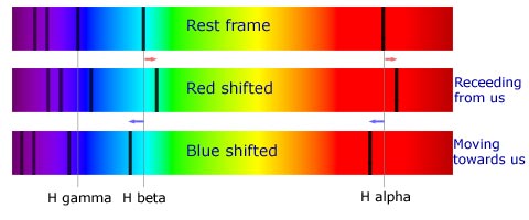Fig 5 : Red Shifted and Blue Shifted spectra compared to a spectrum in rest frame

The Doppler Effect in stellar spectra soon became an important tool to calculate velocities of stars and even galaxies on the cosmological scale. These calculations yielded precise velocities of stars in binary and more complicated star systems. The radial velocity method was used to detect and measure the wobbles produced in a star because of the gravitational tugging of a potential exoplanet. The velocities allowed estimating masses of star in star systems by simple mechanical calculations.

 

In the 20^th century, developments in Quantum Mechanics and Thermodynamics found its applications in the field of Astronomy and Astrophysics. In Thermodynamics, one of the main concerns is the ways in which heat energy can be absorbed or transmitted by a body. You must have noticed whenever you bring your hand close to a heated pan or a piece of metal; you could feel the heat without touching the pan. This is because when the pan gets hot, its molecules and atoms start to jiggle around randomly and emit radiations which are nothing but electromagnetic radiations mostly of the infrared and microwave regions. These radiations are then incident on the atoms of your skin, which absorb them and get excited in turn, producing heat. The amount of heat radiation that a body can absorb depends mostly on its material and shape. In thermodynamics, one imagines an ideal body which could absorb all of radiation incident on it. Such a body is called as “Blackbody”. Although, no object could be regarded completely as a “blackbody”, there are some cases in which an object could be approximated pretty closely as a blackbody. Experiments were conducted with such blackbodies to study their nature and as a result various laws were discovered. The most important of them was the – Wien’s Displacement Law. The law states that the wavelength of the radiation of maximum intensity emitted by a body is inversely proportional to its temperature. A body generally emits electromagnetic radiations in all wavelengths at different intensities. Wien’s law relates the wavelength of this radiation to the temperature of the body. This relation is such that the wavelength of emission is inversely proportional to the body temperature, or the frequency of emitted radiation is directly proportional to the temperature. Consequently, a hot body will emit radiation of higher frequency than that emitted by a cooler one. So, bodies at higher temperatures will glow with a bluish hue and those at cooler temperatures will appear reddish. Alternatively, this result can also be explained by the energy – frequency relation given by Planck, which we saw earlier. Bodies at higher temperatures have more heat energy and hence will glow at higher frequencies and vice versa.

In spectroscopy, this thermodynamic relation was used to estimate the temperature of stars and celestial bodies which emit radiation. The relative brightness of the different colors in a stellar spectrum is compared, and the color with greatest brightness (intensity) is used to calculate the temperature of a star. If the maximum intensity is more towards the bluer side of spectrum, then the star itself appears bluish and has a very high temperature. Similarly, if the maximum intensity is towards the redder side of spectrum then the star has a low temperature. Therefore, a common observation in Astronomy was that red stars are cooler than blue stars. On the basis of their color and respective temperatures, the stars can be classified into different types. This is known as the Harvard Spectral Classification and all the stars are roughly divided into 7 broad categories from hottest to coolest as : O, B, A, F, G, K, M. The stars from O to F are blue or bluish-white in appearance and have a hot temperature of 6000 to above 25,000 kelvins.  The stars from G to M are yellowish white to red in appearance and have a relatively cooler temperature of 3000 to 5000 kelvins. Our Sun belongs to the G type and glows in white color with an intermediate temperature. It appears yellow – orange from Earth due to atmospheric scattering effects.

Fig 6: Spectral curve peak of different stars according to their temperature

What appeared to be a simple result of placing a glass object in the path of light rays was employed so extensively in the domains of Astronomy. A simple glass prism enabled us to calculate the chemical and physical properties of stars at vast distances. Perhaps, one could take this as a prime example for the tremendous potential of seemingly trivial discoveries in Physics. The current state of Modern Physics is often questioned for its benefaction to human society. Nevertheless, I believe that with time and progress, the importance of gravitational waves, particle accelerators, and black holes will soon be realized similar to the importance of the rainbow obtained from a prism.

 

-        Thank you.

 

Lagrangian and Hamiltonian Mechanics : An Unseen Side of Classical Physics

Ever since, school and high-school till the early undergraduate years, students are rigorously made accustomed to the world of Newtonian Mechanics. In fact, those studying in other fields than the Physical Sciences may never see the world beyond this Newtonian Framework of Classical Physics. All of us have been taught and told to remember by heart the three most important laws of Mechanics - Newton's Laws of Motion. These laws provide an intuitive insight to how physical systems evolve and behave with time. They lay down the mathematical foundations to compute the trajectory of any object i.e. its motion through space as time passes, mainly - the Newton's Second Law of Motion which states that the magnitude of an external force experienced by any body is proportional to how much it accelerates. The proportionality constant here is the "inertial mass" of that body. Alternatively, one can say in the language of Calculus that the external force experienced by a body is equal to the product of its mass(m) and the derivative (rate of change) of its velocity with respect to time (dv/dt). But, velocity of that body is the rate of change of its displacement, or the derivative of displacement (x) with respect to time. By this definition, acceleration can be represented by the second derivative of position with respect to time, or - "The rate of change of  the rate of change of position". The first one sounds better.  This renders Newton's Second Law of Motion into a "Differential Equation" which can be solved by special methods. By solving this differential equation, the final solution is obtained in the form of a function x(t). Mapping this function against the time variable on a graph, shows visually how any physical system behaves with time and also predict its future states.

This formulation of Classical Physics works just fine in most scenarios and physical systems. However, there are some systems where applying Newton's formalism becomes too messy and rather inconvenient. Situations such as a double pendulum, a pendulum fixed to a moving support, an object sliding on an inclined plane which itself is moving, etc. are some examples where Newtonian Mechanics isn't a viable option. Such systems either comprise of too many coordinates and independent parameters or too many external forces or both, that it is extremely hard to keep track of individual forces and their effect on other forces. Life would get easier, if somehow it became possible to find our way around this problem by using some other physical quantity to predict the behavior of such dynamic systems. This other way around to the problem manifested itself in the form of Hamiltonian and Lagrangian Mechanics. The formalism was developed by Joseph-Louis Lagrange and Sir William Hamiltonian in the 18th and 19th centuries respectively. 

The core principle behind Lagrangian and Hamiltonian Mechanics is the mathematical concept of Calculus of Variations. The ordinary Calculus most of us are familiar with involves "functions" which is a one to one relation between two real number sets. They can be regarded as machines that take one real number as an input upon which certain mathematical operations act and spew out another or same number as an output. Calculus of Variations on the other hand deals with "Functionals" - they are machines that take an entire function as an input and yield a number as an output. The task in hand is then to minimize these "functionals" subject to certain constraints. A main goal of this article is not to hinge on the abstract mathematics but try to provide an intuition for the idea behind that mathematics. A central quantity of Lagrangian Mechanics is the "Lagrangian Function (L)" or simply the Lagrangian. This Lagrangian is equal to the difference between the Kinetic Energy (T) (yes, Kinetic Energy is represented by T) and the Potential Energy (V).

L = T - V   -- (1)

The integral of this Lagrangian in the limits of the starting time (t1) and ending time (t2) is equal to a quantity called as "Action". This quantity is the example of a "functional" which takes the Lagrangian function as input and gives a number. But where are we headed to by introducing such weird names for some mere mathematical operations on already existing quantities like Kinetic and Potential Energy from Newtonian Physics? Most standard introductory texts on the subject skip this intuition part and dive directly into the complicated derivations of mathematics. What we have here is the Lagrangian Function, which is the difference in Kinetic Energy and Potential Energy. The Kinetic Energy of a system is a direct representation of how much "motion" is happening in that system, while Potential Energy represents how much motion "could" happen in that system but isn't happening. A stretched rubber band or a ball placed on a height packs in more Potential Energy, but if you let go of the rubber band or allow the ball to fall from that height, this Potential Energy is converted to Kinetic Energy. From equation 1 we can infer that, if a system has greater Kinetic Energy its Lagrangian is greater and so the system is more dynamic, more "lively". Conversely, if its Potential Energy is greater then the system is less dynamic, less "lively". The integral (or summation) of this "liveliness"  of a system over some time period gives the "Action" of that system. 

Now, the main principle of Lagrangian Mechanics which is also known as the "Principle of Least Action" says that - the path followed by a system through space between any initial and final time is such that its Action is minimized or remains least. This implies that a system always goes through that path for which its Action is minimal or for which it's "liveliness" or "dynamicity" is least . 

Above diagram visualizes a few of all the possible paths between two points that a system can take while travelling through space and time. There is an infinite number of all such bizarre paths that one can draw. With each of such paths (represented by the different colours) a number is associated with them, which was introduced earlier as "Action". The system starts at point A at time t1 and reaches at point B at time t2.The "Action" of each individual paths between these points is then determined by the different Lagrangians of those paths. Some paths may have a greater Lagrangian value and thus the system going through such paths is more lively and in motion, while some paths have lesser overall Lagrangian and the system is less dynamic for such paths. Out of the seemingly many infinite paths, the Principle of Least Action tells us that this system will take that path for which the "Action' associated with it is least. It is as if there is an algorithm that already dictates what path a system shall choose.

Oddly enough what it means is that Nature is a bit lazy! Initially, this result was somehow attributed to the assertion that God chooses such a path for a system for which the action is minimum. The sense behind this statement is quite pragmatic. If I were to govern the motion of all objects in this Universe, I would most certainly prefer objects to not bounce around much without any reason. Either way, the principle did confirm with observed motions of dynamic bodies. Every spontaneous process in nature minimizes the Action of that process. The most important application of this principle was to explain the behavior of light. Fermat's principle which was a modified analog of Hamiltonian and Lagrangian Mechanics accounted for the path taken by any light ray, which is such that the time taken to travel between two points is minimized. By working through the Principle of Least Action, one arrives at the Euler - Lagrange Equation - An epitome of Lagrangian Mechanics. This equation represents Lagrangian Mechanics in the same way that F = ma represents Newtonian Mechanics. In fact, it is very much possible to extract the mathematical statement of Newton's Second Law from the Principle of Least Action and Euler - Lagrange Equation, even if the two appear distinct.

The above equation is the Euler - Lagrange Equation. It can be classified as a second order differential equation. The letter q in it represents the "generalized coordinate". Here generalized meaning that the coordinate can refer to anything. For example, one can use cartesian coordinates in case of linear motion, or polar coordinates for a pendulum or angular motion, etc. The fancy L like letter, is the symbolic representation of our Lagrangian Function given by :

Lagrangian is a function of the generalized coordinate q and the velocity of system, which is represented by the second q with a dot overhead. A convention in Physics is to denote the rate of change of a quantity(derivative) with respect to time by placing a dot over it. In the 19th century, Hamilton developed a similar modified version of Lagrangian Mechanics that became known as Hamiltonian Mechanics. Just like the Lagrangian, his version involves a "Hamiltonian" which is equal to the sum of Kinetic and Potential Energies of a system. 

H = T + V   --(4)

The Hamiltonian Equations of motion are :

Here q is the generalized coordinate and p is the momentum of system.

Lagrangian Mechanics along with Hamiltonian Mechanics proved crucial in supplementing the mathematics of modern Physics. The Hamiltonian became an operator which is extensively used in Schrodinger's Equation. The Principle of Least Action along with Lagrangian Mechanics was employed by Richard Feynman in his Path Integral Formulation of Quantum Physics. The Lagrangian is even found in Quantum Field Theory - one of the most precise theory ever discovered by mankind. Unfortunately, Lagrangian and Hamiltonian Mechanics wasn't able to gain the fame and recognition that Newton's Laws did in everyday lives. This could be explained perhaps by the fact that a physical intuition for these formulations is hard to explain. But, sometimes the physical intuition behind a theory isn't the most significant aspect as long as it works consistently, which is the case for Lagrange and Hamilton's theories.

- Thank You.